11 Colour scales and legends

11.1 Exercises

drv_labels <- c("4" = "4wd", "f" = "fwd", "r" = "rwd")

ggplot(mpg, aes(displ, hwy)) + 
  geom_point(aes(colour = drv)) +
  scale_colour_discrete(labels = drv_labels)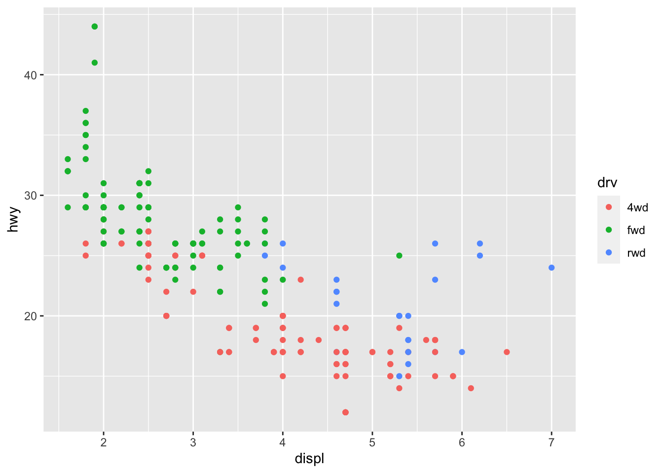

• We store the labels inside drv_labels and use it in scale_colour_discrete()

11.2 Exercises

1. How do you make legends appear to the left of the plot? -theme(legend.position = “left”)make legends appear to the left of the plot. - Other options:theme(legend.position = “right”),theme(legend.position = “bottom”), andtheme(legend.position = “none”)`

2. What’s gone wrong with this plot? How could you fix it?

• There are two separate legends for the same variable (drv). We need to combine these two legends into one. To do this, both color and shape need to be given shape specifications.

ggplot(mpg, aes(displ, hwy)) + 
  geom_point(aes(colour = drv, shape = drv)) + 
  scale_colour_discrete("Drive train",
                        breaks = c("4", "f", "r"),
                        labels = c("4-wheel", "front", "rear")) +
  scale_shape_discrete("Drive train",
                        breaks = c("4", "f", "r"),
                        labels = c("4-wheel", "front", "rear"))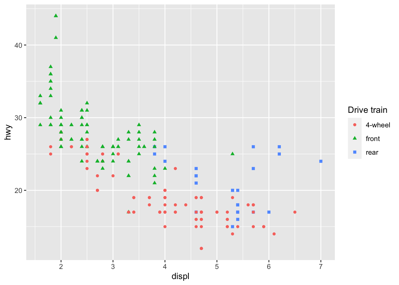

3.

ggplot(mpg, aes(displ, hwy, colour = class)) + 
      geom_point(show.legend = FALSE) + 
      geom_smooth(method = "lm", se = FALSE) + 
      theme(legend.position = "bottom") + 
      guides(colour = guide_legend(nrow = 1))
#> `geom_smooth()` using formula 'y ~ x'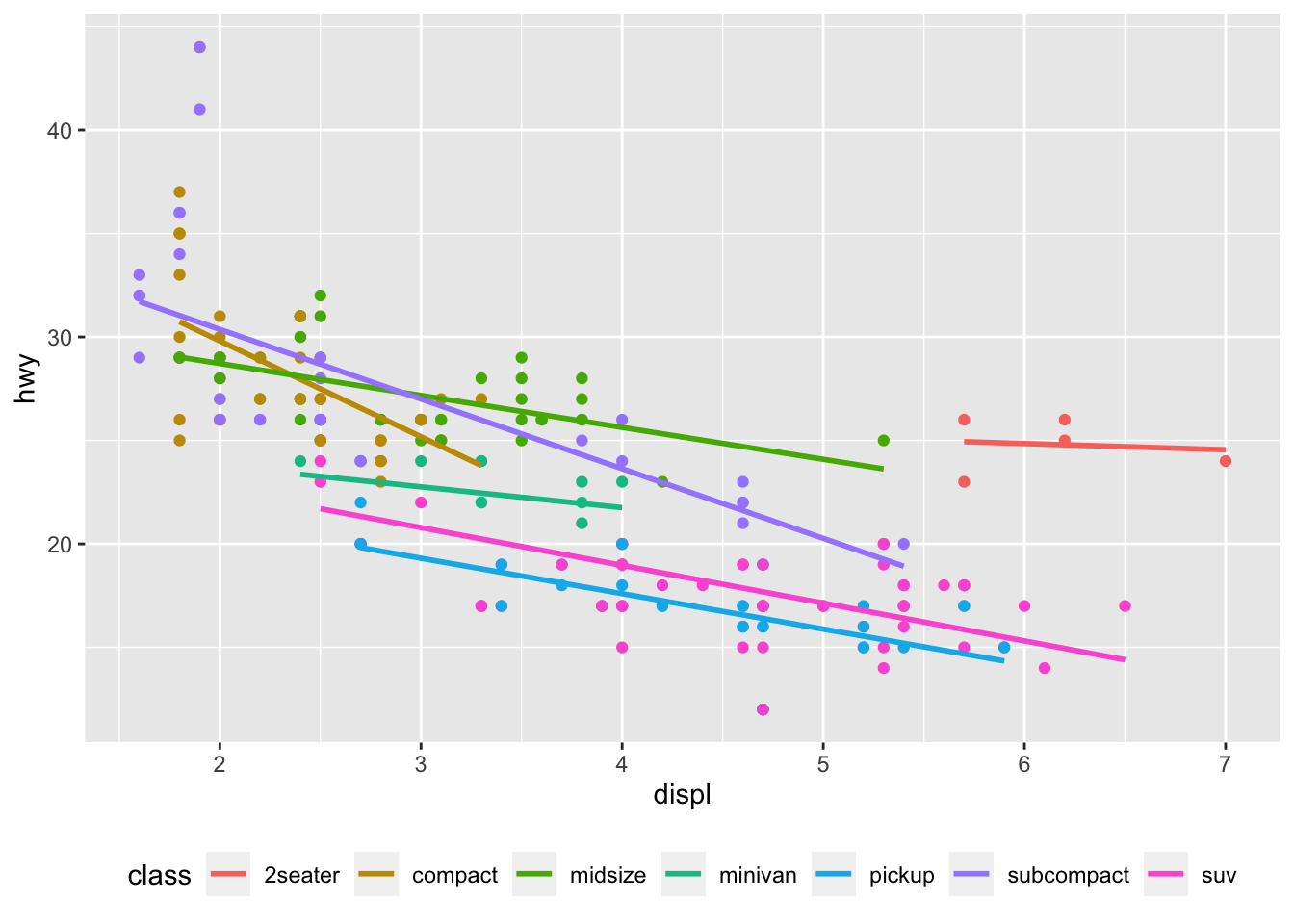

Note: The answers to these “recreate the code for this plot” questions are provided in the source code of the book.